Multiple linear regression
(Andrea Zagaria)
keywords multiple regression, 2SLS, instrumental variables regression, jamovi
In this example we show how to implement an instrumental variable regression via two stage least-squares (2SLS) estimation using ENDOj.
Introduction
Ordinary least squares (OLS) linear regression assumes that independent variables are uncorrelated with the outcome’s error term (Wooldridge, 2006). When this assumption is violated, e.g., due to the omitted variable bias, simultaneous causality or measurement error, OLS estimates may be inconsistent (Stock & Watson, 2015). A predictor variable that correlates with the error term in a regression equation is called an endogenous variable. Several methods have been proposed to deal with endogeneity issues within a linear regression framework, such as the so-called instrumental variable (IV) methods (Stock & Watson, 2015). ENDOj package implements the IV method via the two-stage least-squares (2SLS) estimation, the most common IV estimator (Bascle 2008; Bollman et al., 2019). 2SLS requires the use of external variables, also defined instrumental variables, that are outside the proposed model. Specifically, an instrumental variable has the aim to disentangle the portion of the endogenous variable that is not correlated with the outcome’s error term (i.e., first step), therefore using this predicted portion to explain the criterion variable (i.e., second step) (see Bollmann et al., 2019 for a theoretical illustration). To consistently interpret findings from 2SLS, the instrumental variable should be correlated with the endogenous variable (i.e., the instrument relevance condition) but not with the error term of the model (i.e., the instrument exogeneity condiction, also known as the ortogonality condiction) (Stock & Watson, 2015).
Simulated example
To demonstrate how ENDOj work, we propose the following example based on a simulated dataset composed of 350 participants, each with 5 observed variables: age, the average number of cigarettes smoked daily (smoking); caloric intake before bedtime (calorie), insomnia symptoms (insomnia), academic performance (academic). They are all treated as continuous variables.
The aim is threefold: (1) test the hypothesized regression model through the standard OLS regression; (2) address potential endogeneity issues by implementing an IV regression via 2SLS estimation; (3) compare findings from these two approaches.
Let’s assume we want to estimate the predictive role of insomnia symptoms on academic performance whilst controlling for age differences.
OLS linear regression
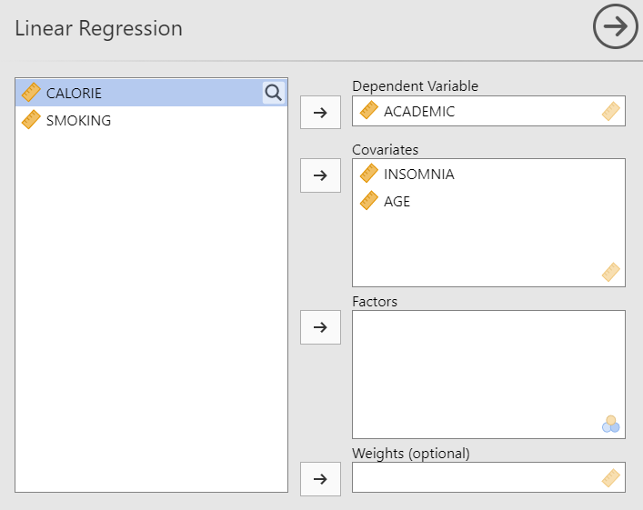
First, we implement a multiple regression model through the standard OLS approach defining academic as a criterion variable, while insomnia and age are inserted as predictor variables.
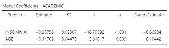
The B coefficients are found in the “Model coefficients” table. This table basically shows that the partial standardized regression coefficient linking insomnia to academic is -.669, p<.001. Hence, a change of 1 standard deviation in insomnia is associated with a change of -.669 standard deviations in academic.
Two-stages least-squares estimation (2SLS)
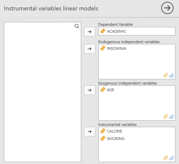
Afterwards, we re-run the analysis through the ENDOj package addressing potential endogeneity issues of insomnia (i.e., the case in which insomnia symptoms correlate with the error term of the regression equation) via the 2SLS approach. For the purpose of this example, we define the average number of cigarettes smoked daily (smoking) and the calorie intake before bedtime (calorie) as external instrumental variables, since both factors have been associated with sleep interference. Age is still defined as a covariate and used as instruments for itself.
The first table of interest is the “Model diagnostics” table which summarizes the diagnostic tests for endogeneity.
The Weak instruments test examines the null hypothesis that the instrumental variables are weakly correlated with the endogenous variable (i.e., insomnia). A significant p-value sustains the alternative hypothesis that the instrument is strong (see Stock & Watson, 2015), also ensuring the satisfaction of the instrument relevance condition.
The Wu-Hausman’s specification test examines the null hypothesis that insomnia is exogenous. A significant p-value, as in the example, provided evidence that insomnia is truly endogenous and, therefore, that the 2SLS approach is recommended over the standard OLS regression.
The Sargan’s test examines the null hypothesis that the instrumental variables are not correlated with the regression error term. A significant p-value suggests that the instruments do not meet the exogeneity condition.
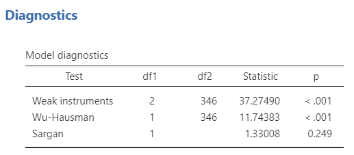
The model diagnostics suggest that insomnia is truly endogenous, thus the implementation of the 2SLS estimation is justified. Also, the instrumental variables correlate with the endogenous variable but not with the regression error term, satisfying the relevance condition and the exogeneity condition, respectively.
The B coefficients obtained from the 2SLS approach can be found in the “Parameters Estimates” table. ENDOj provide non-standardized and standardized estimates, standard errors and 95% confidence intervals for each coefficient. As can we see, the partial standardized regression coefficient linking insomnia to academic is now -.379, p<.001. Accordingly, a change of 1 standard deviation in insomnia is associated with a change of -.379 standard deviations in academic.
Note that robust standard errors, as well as confidence intervals through the bootstrap approach can be requested by ticking these options in the “Model options” panel.
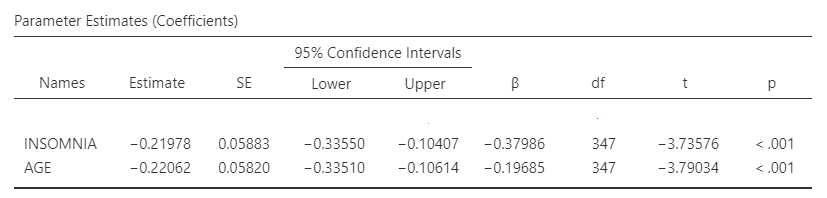
Comparing the 2SLS parameters with the OLS parameters, we observe that the 2SLS regression coefficient (β=-.379) is far below in size as opposed to the coefficient obtained from standard OLS regression (β=-.669), demonstrating how the latter estimate is inconsistent and upward biased. We can also notice that the standard errors of the coefficients are larger for 2SLS approach than for standard OLS.
References
Bascle, G. (2008). Controlling for endogeneity with instrumental variables in strategic management research. Strategic organization, 6(3), 285-327.
Bollmann, G., Rouzinov, S., Berchtold, A., & Rossier, J. (2019). Illustrating instrumental variable regressions using the career adaptability–job satisfaction relationship. Frontiers in Psychology, 10, 1481.
Stock, J. H., & Watson, M. W. (2015). Introduction to econometrics. London: Pearson
Wooldridge, J. M. (2006) Introductory Econometrics: A Modern Approach, 3rd edn. Mason, OH: Thomson-South Western.