Simple linear regression
(Andrea Zagaria)
keywords simple regression, 2SLS, instrumental variables regression, jamovi
In this example we show how to implement an instrumental variable regression via two stage least-squares (2SLS) estimation using ENDOj.
Introduction
Ordinary least squares (OLS) linear regression assumes that independent variables are uncorrelated with the outcome’s error term (Wooldridge, 2006). When this assumption is violated, e.g., due to the omitted variable bias, simultaneous causality or measurement error, OLS estimates may be inconsistent (Stock & Watson, 2015). A predictor variable that correlates with the error term in a regression equation is called an endogenous variable. Several methods have been proposed to deal with endogeneity issues within a linear regression framework, such as the so-called instrumental variable (IV) methods (Stock & Watson, 2015). ENDOj package implements the IV method via the two-stage least-squares (2SLS) estimation, the most common IV estimator (Bascle 2008; Bollman et al., 2019). 2SLS requires the use of external variables, also defined instrumental variables, that are outside the proposed model. Specifically, an instrumental variable has the aim to disentangle the portion of the endogenous variable that is not correlated with the outcome’s error term (i.e., first step), therefore using this predicted portion to explain the criterion variable (i.e., second step) (see Bollmann et al., 2019 for a theoretical illustration). To consistently interpret findings from 2SLS, the instrumental variable should be correlated with the endogenous variable (i.e., the instrument relevance condition) but not with the error term of the model (i.e., the instrument exogeneity condiction, also known as the ortogonality condiction) (Stock & Watson, 2015).
Example of a two-stages least-squares estimation (2SLS)
To demonstrate how ENDOj work, we analysed data provided and described in the ivreg package as SchoolingReturns (https://cran.r-project.org/web/packages/ivreg/vignettes/ivreg.html). The dataset is taken from the supplementary material for Verbeek (2004) and is based on the work of Card (1995).
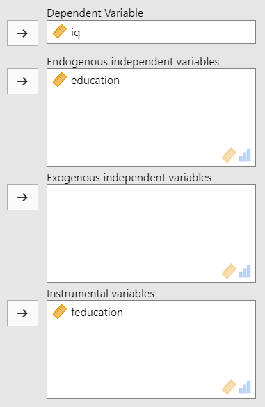
We aimed to investigate the impact of scholing on intelligent quotient by implementing an IV regression via 2SLS estimation. Schooling (education) was defined as a predictor variable. The intelligent quotient (IQ) was defined as a criterion variable. Within a standard OLS regression, this estimate may be problematic, since it can be argued that education may suffer from endogeneity issues (i.e., it may be correlated with the regression error term). By employing a 2SLS estimation, we defined father’s education (feducation) as the natural exogenous instrument for education. To fit this model, we can simply follow the indications represented below:
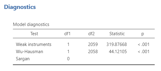
The first table of interest is the “Model diagnostics” table which summarizes the diagnostic tests for endogeneity.
The Weak instruments test examines the null hypothesis that the instrumental variable (i.e., feducation) is weakly correlated with the endogenous variable (i.e., education). A significant p-value, as in this example, sustains the alternative hypothesis that the instrument is strong (see Stock & Watson, 2015), also ensuring the satisfaction of the instrument relevance condition.
Wu-Hausman’s specification test examines the null hypothesis that education satisfies the exogeneity assumption. A significant p-value, as in the example, sustains the alternative hypothesis that education suffers from endogeneity and, therefore, that the 2SLS approach is recommended over the standard OLS regression.
With respect to Sargan’s test, note that since the model is just-identified the statistic cannot be computed. For a just-identified model, it is non-viable to formally test whether the instrumental variables are exogenous (see Stock & Watson, 2015).
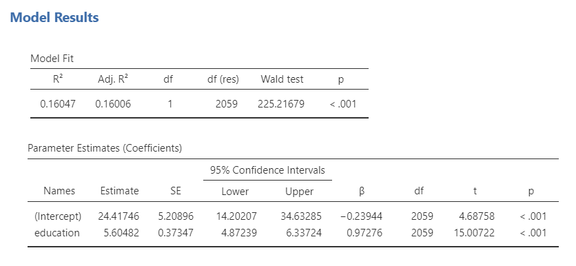
Let’s take a look at the “Model results” paragraph. We highlighted that the unstandardized regression coefficient linking education to IQ was 5.604, whilst the standardized regression coefficient was 0.972, p<.001. It basically means that for each 1-unit increment of education, IQ is expected to increase by 5.604. With regards to the standardized coefficient, a change of 1 standard deviation in education is associated with a change of 0.972 standard deviations in IQ. Moreover, the regression model explained approximately 16% of the variance of IQ,
Note that robust standard errors, as well as confidence intervals through the bootstrap approach can be requested by ticking these options in the “Model options” panel.
References
Bascle, G. (2008). Controlling for endogeneity with instrumental variables in strategic management research. Strategic organization, 6(3), 285-327.
Bollmann, G., Rouzinov, S., Berchtold, A., & Rossier, J. (2019). Illustrating instrumental variable regressions using the career adaptability–job satisfaction relationship. Frontiers in Psychology, 10, 1481.
Card, D. (1995). Using Geographical Variation in College Proximity to Estimate the Return to Schooling. In: Christofides, L.N., Grant, E.K., and Swidinsky, R. (eds.), Aspects of Labour Market Behaviour: Essays in Honour of John Vanderkamp, University of Toronto Press, Toronto, 201-222.
Stock, J. H., & Watson, M. W. (2015). Introduction to econometrics. London: Pearson
Verbeek, M. (2004). A Guide to Modern Econometrics, 2nd ed. John Wiley.
Wooldridge, J. M. (2006) Introductory Econometrics: A Modern Approach, 3rd edn. Mason, OH: Thomson-South Western.